BitNet b1.58-2B4T: Revolutionary Binary Neural Network for Efficient AI

Archive Paper Link

BitNet b1.58-2B4T: The Future of Efficient AI Processing

A History of 1 bit Transformer Model

A paper “The Era of 1-bit LLMs: All Large Language Models are in 1.58 Bits” was published by Stanford University, ETH Zürich, and EPFL. It was published on October 2023 (published on arXiv on October 17, 2023). Standord Paper Link. The core Concept of 1.58 bits per parameter, was introduced here. This demonstrated that LLMs could be effectively trained and operated with extremely low-bit representation while maintaining competitive performance

Key Difference between 2 Papers

• Different Research Teams: The original BitNet came from academic institutions, while the newer BitNet b1.58-2B4T comes from Microsoft Research
• Technical Advancements: The Microsoft paper builds upon the original concept but adds significant technical improvements:
  • Uses 2-bit activations instead of traditional higher-precision activations
  • Implements 4-bit training methodology for better convergence
  • Likely offers improved performance while maintaining the core 1.58-bit weight approach

There’s approximately a 6-month gap between the papers, with Microsoft’s implementation representing the next evolution of the concept. This situation represents a common pattern in AI research where an innovative concept (in this case, BitNet’s 1.58-bit paradigm) is introduced by one team and then rapidly improved upon by industry research labs with additional resources and engineering capabilities.

Approach taken by Microsoft

Based on the information in the paper sources, the development of BitNet b1.58 2B4T involved several key techniques, which can be broken down step by step in terms of architecture, training, and inference:

1. Architecture Modifications Based on the Transformer Model:

• BitNet b1.58 2B4T’s architecture is derived from the standard Transformer model.
• The core innovation lies in replacing standard full-precision linear layers with custom BitLinear layers.

2. BitLinear Layer Implementation:

• Weight Quantization: During the forward pass, model weights are quantized to 1.58 bits using an absolute mean (absmean) quantization scheme, mapping weights to ternary values {-1, 0, +1}.
• Activation Quantization: Activations flowing through the linear projection are quantized to 8-bit integers using an absolute maximum (absmax) quantization strategy, applied per-token.
• Normalization: Subln normalization was incorporated to enhance training stability, which is particularly beneficial in quantized training.

3. Integration of Established LLM Techniques:

• Activation Function (FFN): Instead of SwiGLU, the model uses squared ReLU (ReLU2) within the feed-forward network sub-layers, motivated by its potential to improve sparsity and computational characteristics in the 1-bit context.
• Positional Embeddings: Rotary Position Embeddings (RoPE) are used to inject positional information, a standard practice in modern LLMs.
• Bias Removal: All bias terms are removed from the linear layers and normalization layers throughout the network to reduce parameter count and potentially simplify quantization.
• Tokenization: The tokenizer developed for LLaMA 3 is adopted, which implements a byte-level Byte-Pair Encoding (BPE) scheme with a vocabulary size of 128,256 tokens.

4. Three-Phase Training Process:

• The training involved three distinct phases: large-scale pre-training, followed by supervised fine-tuning (SFT), and then direct preference optimization (DPO).

5. Pre-training:

• General Training Strategies: Adapted from established LLM practices, with specific adjustments for the 1-bit architecture.
• Learning Rate Schedule: A two-stage learning rate schedule was employed.
  • Stage 1 (High Learning Rate): A standard cosine decay schedule starting with a relatively high peak learning rate, leveraging the observed greater training stability of 1-bit models.
  • Stage 2 (Cooldown): Approximately midway through training, the learning rate was abruptly decayed and subsequently maintained via a cosine schedule with a significantly lower peak value to refine representations on higher-quality data.
• Weight Decay Schedule: A two-stage weight decay strategy was implemented.
  • Stage 1: Weight decay followed a cosine schedule, reaching a peak value of 0.1 to help prevent overfitting during the initial high-learning-rate phase.
  • Stage 2: Weight decay was effectively disabled (set to zero) to allow the model parameters to settle into finer-grained optima guided by the lower learning rate and curated data.
• Pre-training Data: A mixture of publicly available text and code datasets, including DCLM and FineWeb-EDU, along with synthetically generated mathematical data to enhance reasoning abilities. Data presentation aligned with the two-stage training, with general web data in Stage 1 and higher-quality curated datasets in Stage 2.

6. Supervised Fine-tuning (SFT):

• SFT Data: A diverse collection of publicly available instruction-following and conversational datasets, including WildChat, LMSYS-Chat-1M, WizardLM Evol-Instruct, and SlimOrca, supplemented with synthetic datasets generated using methodologies like GLAN and MathScale to bolster specific capabilities.
• Chat Template: A specific chat template structure was used for conversational tasks.
• Optimization Details:
  • Loss Aggregation: Summation of the cross-entropy loss across tokens within a batch was used instead of averaging, which empirically improved convergence and final performance.
  • Hyperparameter Tuning: Careful tuning of the learning rate (relatively larger than typical for full-precision models) and the number of training epochs (extended duration required for optimal convergence) was performed.

7. Direct Preference Optimization (DPO):

• Training Data: A preference dataset constructed from a combination of publicly available resources, specifically UltraFeedback and MagPie.
• Training Details: Conducted for 2 epochs with a learning rate of 2× 10−7 and a DPO beta parameter of 0.1. Optimized kernels from the Liger Kernel library were integrated to enhance training efficiency.

8. Inference Implementation:

• Dedicated inference libraries were developed and open-sourced for both GPU and CPU platforms to handle the unique W1.58A8 quantization scheme.

9. GPU Inference:

• A custom CUDA kernel was specifically designed for the W1.58A8 matrix multiplication since standard libraries lack optimized kernels for this mixed-precision, low-bit format.
• The kernel employs a ‘pack-store-load-unpack-compute’ strategy for weights. Four ternary weight values are packed into a single 8-bit integer for storage in HBM. During computation, they are loaded into faster SRAM, unpacked, and then used for matrix multiplication with 8-bit activations.

10. CPU Inference:

• The bitnet.cpp library was developed as an official reference implementation for CPU inference of 1-bit LLMs, including BitNet b1.58.
• Optimized kernels tailored for standard CPU architectures were implemented to work efficiently with the model’s quantization scheme, ensuring numerical accuracy relative to the training procedure (lossless inference).

These steps outline the core techniques employed in the research and development of BitNet b1.58 2B4T.

Key Concepts

Based on the information in the sources, here are some YouTube friend keywords that could be relevant to this research paper on BitNet b1.58 2B4T:

• BitNet b1.58 2B4T: This is the specific name of the model and a key identifier for the research.
• 1-bit LLM: This highlights the core characteristic of the model as a 1-bit Large Language Model.
• Large Language Model: This is the broader category of AI models the research falls under.
• Efficient LLM: The paper emphasizes the computational efficiency of BitNet b1.58 2B4T.
• Low-bit LLM: This is another way to describe models with reduced precision, like the 1.58-bit weights used in BitNet b1.58 2B4T.
• Native 1-bit training: The model is trained from scratch with 1-bit weights, which is a key distinction from post-training quantization.
• Model Quantization: This is the technique of reducing the precision of model weights and activations, central to the research.
• Hugging Face: The model weights are released on Hugging Face, making it a relevant platform for discussion and collaboration.
• Open-source LLM: BitNet b1.58 2B4T is the first open-source native 1-bit LLM at its scale.
• GPU inference optimization: The paper discusses custom CUDA kernels for efficient GPU inference.
• CPU inference for LLMs: The development of bitnet.cpp for CPU inference is a significant aspect of the work.
• bitnet.cpp: This is the name of the open-source C++ library for CPU inference of 1-bit LLMs.
• Transformer architecture: BitNet b1.58 2B4T’s architecture is derived from the standard Transformer model.
• Memory efficient AI: The reduced memory footprint is a major advantage of BitNet b1.58 2B4T.
• Energy efficient AI: Lower energy consumption is another key benefit highlighted in the paper.
• Fast inference LLM: The model offers potentially lower decoding latency.
• LLM benchmarks: The paper evaluates the model on various benchmarks for language understanding, reasoning, math, and code.
• Performance vs Efficiency LLM: The research aims to bridge the gap between performance and efficiency in large language models.
• AI for edge devices: The efficiency of 1-bit LLMs makes them potentially suitable for resource-constrained environments.

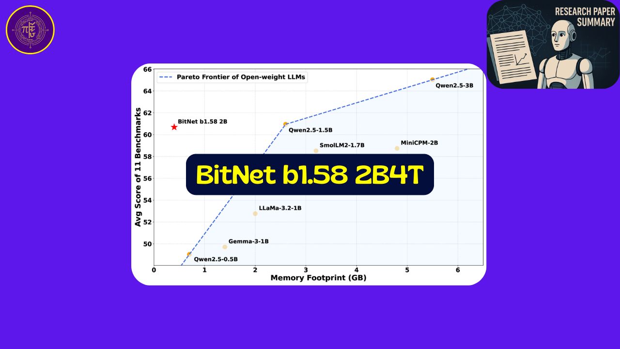
Benchmark comparisons

As per the paper comparision of 1.58bit model with Others is as below.

General Performance Metrics

Benchmark (Metric)	LLaMA 3.2	Gemma-3	Qwen2.5	SmolLM2	MiniCPM	BitNet b1.58
Parameters	1B	1B	1.5B	1.7B	2B	2B
Memory (Non-emb)	2GB	1.4GB	2.6GB	3.2GB	4.8GB	0.4GB
Latency (CPU; TPOT)	48ms	41ms	65ms	67ms	124ms	29ms
Energy (Estimated)	0.258J	0.186J	0.347J	0.425J	0.649J	0.028J
Training Tokens (Pre-training)	9T (pruning & distillation)	2T (distillation)	18T	11T	1.1T	4T

Dataset Specific Metrics

Model - # of Paramerters Databaset / Benchmark (Metric)	LLaMA 3.2 (1B)	Gemma-3 (1B)	Qwen2.5 (1.5B)	SmolLM2 (1.7B)	MiniCPM (2B)	BitNet b1.58 (2B)
ARC-Challange (0-shot; Acc,norm)	37.8	38.4	46.67	43.52	44.8	49.91
ARC-Easy (0-shot; Acc,norm)	63.17	63.13	76.01	62.92	72.14	74.79
OpenbookQA (0-shot; Acc,norm)	34.8	38.8	40.8	46	40.2	41.6
BoolQ (0-shot; Acc)	64.65	74.22	78.04	75.78	80.67	80.18
HellaSwag (0-shot; Acc,norm)	60.8	57.69	68.28	71.71	70.81	68.44
PIQA (0-shot; Acc,norm)	74.21	71.93	76.12	76.12	76.66	77.09
WinoGrande (0-shot; Acc)	59.51	58.48	62.83	68.98	61.8	71.9
CommonsenseQA (10-shot; Acc)	58.48	42.1	76.41	63.55	71.74	71.58
TruthfulQA (10-shot; MC2)	43.8	38.66	46.67	39.9	41.41	45.31
TriviaQA (5-shot; EM)	37.6	23.49	38.37	45.97	34.13	33.57
MMLU (5-shot; Acc)	45.58	39.91	60.25	49.24	51.82	53.17

### Niche Datasets

Model - # of Paramerters Databaset / Benchmark (Metric)	LLaMA 3.2 (1B)	Gemma-3 (1B)	Qwen2.5 (1.5B)	SmolLM2 (1.7B)	MiniCPM (2B)	BitNet b1.58 (2B)
HumanEval+ (0-shot; Pass@1)	31.1	37.2	50.6	28	43.9	38.4
GSM8K (4-shot; EM)	38.21	31.16	56.79	45.11	4.4	58.38
MATH-500 (0-shot; EM)	23	42	53	17.6	14.8	43.4
IFEval (0-shot; Instruct-Strict)	62.71	66.67	50.12	57.91	36.81	53.48
MT-bench (0-shot; Average)	5.43	6.4	6.12	5.5	6.57	5.85
Average	44.9	43.74	55.23	48.7	42.05	54.19

• HumanEval is a benchmark dataset created by OpenAI to evaluate the performance of large language models (LLMs) in code generation tasks
• The GSM8K benchmark comprises 1,319 grade school math word problems, each crafted by expert human problem writers. These problems involve elementary arithmetic operations (+ − ×÷) and require between 2 to 8 steps to solve.
• IFEval dataset evaluates instruction following ability of large language models. There are 500+ prompts with instructions such as “write an article with more than 800 words”, “wrap your response with double quotation marks”
• Multi-turn benchmark (MT-Bench) is a novel evaluation framework that tests the conversational capabilities of language models.

Applications of BitNet b1.58-2B4T Architecture

Based on the binary neural network architecture of BitNet b1.58-2B4T, here are the most promising applications where this state-of-the-art model could make significant impact:

Edge Computing Applications

• IoT Sensors and Devices: BitNet can enable complex NLP capabilities on resource-constrained IoT devices that previously couldn’t support traditional language models
• Smart Home Systems: Local processing of voice commands and text without cloud dependencies
• Wearable Technology: Enhanced on-device language understanding for smartwatches and health monitors

Mobile Applications

• On-Device Translation: Real-time translation without internet connectivity
• Content Recommendation: Personalized content filtering that preserves privacy by keeping data on-device
• Voice Assistants: More capable mobile assistants with reduced cloud dependence

Enterprise Solutions

• Cost-Efficient NLP Infrastructure: Organizations can deploy advanced language capabilities with reduced hardware requirements
• Scalable Language Processing: Process more requests with existing hardware infrastructure
• Energy-Efficient Data Centers: Significant power consumption reduction for large-scale deployments

Privacy-Focused Applications

• Healthcare Data Analysis: Process sensitive medical information locally without transmitting to cloud services
• Financial Services: Analyze transactions and detect fraud patterns on-device
• Confidential Document Processing: Enterprise document analysis without exposing data to external servers

Resource-Constrained Environments

• Embedded Systems: Industrial control systems with advanced language capabilities
• Robotics: More sophisticated language understanding for robots with limited computing power
• Remote/Rural Applications: AI capabilities in areas with limited connectivity or power

Sustainability Applications

• Carbon Footprint Reduction: Lower energy requirements for AI deployments
• Longer Battery Life: Extend operational time of mobile and edge devices
• Sustainable AI Deployment: Enable AI capabilities in green computing initiatives

These applications leverage BitNet’s core advantages: dramatically reduced computing requirements while maintaining performance comparable to much larger models, enhanced privacy through local processing, and significant cost and energy efficiency improvements.

For your SEO strategy, highlighting these specific applications with real-world examples would help attract readers interested in practical implementations rather than just the technical architecture.

What is Weight Quantization?

Weight quantization is a technique used to reduce the size and computational cost of a neural network by representing weights with fewer bits.

In this case:

• Weights are quantized to 1.58 bits → that’s an average bit-per-weight, which implies ternary quantization (3 possible values).
• The quantized values are { -1, 0, +1 }.
• The method used is absolute mean (absmean) quantization.

---

🔍 What’s “absmean” quantization?

This scheme sets thresholds based on the mean of the absolute values of the weights in a layer or tensor.

Here’s the general process:

1. Calculate T = mean(abs(weights)) (the absmean threshold).
2. For each weight w:
   • If w > T, set it to +1.
   • If w < -T, set it to -1.
   • If -T ≤ w ≤ T, set it to 0.

---

🧮 Example: Quantizing a Tensor

Let’s say you have a simple weight tensor:

weights = [-2.0, -0.5, 0.0, 0.3, 1.2, 2.5]

Step 1: Compute absmean

absmean = mean(abs(weights)) = mean([2.0, 0.5, 0.0, 0.3, 1.2, 2.5]) = 6.5 / 6 ≈ 1.083

Step 2: Apply absmean quantization

quantized_weights = []
for w in weights:
    if w > 1.083:
        quantized_weights.append(+1)
    elif w < -1.083:
        quantized_weights.append(-1)
    else:
        quantized_weights.append(0)

Output:

weights =     [-2.0, -0.5, 0.0, 0.3, 1.2, 2.5]
quantized =   [ -1 ,   0 ,  0 ,  0 ,  1 ,  1 ]

Now the weights are ternary: {-1, 0, +1} — with each weight approximated using only log₂(3) ≈ 1.58 bits. Why log2 and not lo10? Because our digital system uses 0,1. Why 3 and not 5 or 7? Because we are using 3 values (-1,0,1).

---

✅ Why is this useful?

• Memory savings — from 32-bit float to ~1.58 bits.
• Faster inference — multiply becomes add/subtract or skip (for zero).
• Sparsity — 0 weights can be skipped during computation.

What is SubLN (Sub-layer Normalization)

SubLN (Sublayer Normalization) is a variant of normalization applied within sublayers of a neural network (like Transformer layers), after the residual connection and before the activation function. It stabilizes the learning process.

It Reduces quantization noise, Stabilizes training, Improves convergence, Applies after residual, Common in Transformers

It’s similar in spirit to LayerNorm but usually simpler and more efficient, especially helpful for low-precision training, like in quantized models.

---

🧠 Why is this important in Quantized Training?

Quantized weights (e.g., { -1, 0, +1 }) lead to:

• Lower dynamic range
• Noisy gradients
• Instability during training

SubLN:

• Reduces activation noise caused by weight quantization
• Normalizes the outputs of each sublayer, which can vary wildly in quantized settings
• Improves gradient flow and convergence

---

📌 Where is SubLN applied?

In a Transformer-style model:

       Input
         |
     +---+---+
     |       |
     | Self-Attn
     |       |
     +---+---+
         |
      Add + SubLN
         |
     +---+---+
     |       |
     |  MLP
     |       |
     +---+---+
         |
      Add + SubLN
         |
      Output

Each block has:

• Residual Add
• SubLN normalization
• Activation/next layer

---

🧮 Example (PyTorch-style pseudocode)

Let’s say you’re building a Transformer sublayer:

import torch
import torch.nn as nn

class SubLNTransformerBlock(nn.Module):
    def __init__(self, d_model):
        super().__init__()
        self.self_attn = nn.MultiheadAttention(d_model, num_heads=8)
        self.norm1 = nn.LayerNorm(d_model, elementwise_affine=True)
        self.ffn = nn.Sequential(
            nn.Linear(d_model, d_model * 4),
            nn.ReLU(),
            nn.Linear(d_model * 4, d_model),
        )
        self.norm2 = nn.LayerNorm(d_model, elementwise_affine=True)

    def forward(self, x):
        # Self-attention sublayer
        attn_out, _ = self.self_attn(x, x, x)
        x = x + attn_out                  # Residual Add
        x = self.norm1(x)                 # SubLN after residual

        # Feedforward sublayer
        ffn_out = self.ffn(x)
        x = x + ffn_out                   # Residual Add
        x = self.norm2(x)                 # SubLN after residual
        return x

This is essentially implementing SubLN — even though LayerNorm is used, the key is where it’s applied (after residual, before activation or next sublayer).

Hashtags

#BitNetAI #BinaryNeuralNetworks #EfficientAI #EdgeComputing #AIOptimization #LowBitAI #ResourceEfficientML #AIModelCompression #ModelQuantization #AIinference #GreenAI #SustainableML #TinyML #EdgeAI #AIEngineering