Distances in Machine Learning

Distances in Machine Learning

Every sample, record, word, sentence, object, image etc in the Machine learning language is called vector. If we want to measure the similarity or dissimilarity between two data points then we need distance function.

Distance metrics play a crucial role in various machine learning algorithms, including clustering, classification, and anomaly detection. Different distance measures capture different types of relationships between data points.

The choice of distance function depends on the specific task at hand and the properties of the data. For example,

• the Euclidean distance is often used for tasks such as classification and regression,
• the Jaccard distance is often used for tasks such as text classification,
• the Mahalanobis distance is often used for tasks such as fraud detection.
• the Manhattan distance is often used for tasks such as clustering.

1. Manhattan Distance (L1 Norm):

This is the sum of the absolute values of the vector components. It’s called the Manhattan distance because it represents the distance between two points in a grid-based path (like navigating streets in a city laid out in a grid).

\[\| \mathbf{x} \|_1 = |x_1| + |x_2| + \ldots + |x_n|\]

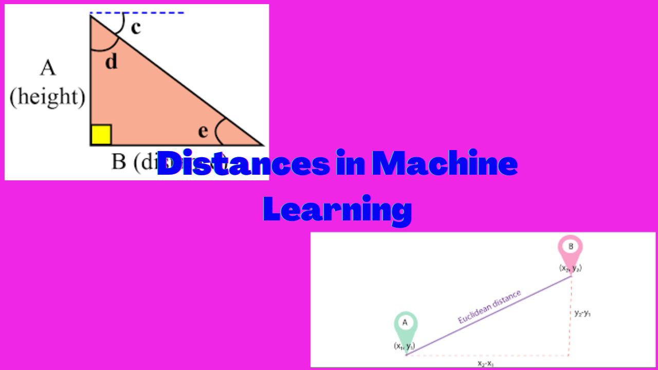
Euclidean Distance(L2 Norm):

This is the square root of the sum of the squares of the vector components. It corresponds to the straight-line distance (or Euclidean distance) between two points in Euclidean space.

\[\| \mathbf{x} \|_2 = \sqrt{x_1^2 + x_2^2 + \ldots + x_n^2}\]

2. Minkowski distance:

This is a generalization of the Euclidean and Manhattan distances. It is defined by a parameter p, and the value of p determines the type of distance metric. For example, p=1 is the Manhattan distance, p=2 is the Euclidean distance, and p=infinity is the Chebyshev distance.

\[\| \mathbf{x} \|_3 = \left(|x_1|^3 + |x_2|^3 + \ldots + |x_n|^3\right)^{\frac{1}{3}}\]

In general, the Lp norm is defined as:

\[\| \mathbf{x} \|_p = \left(|x_1|^p + |x_2|^p + \ldots + |x_n|^p\right)^{\frac{1}{p}}\]

where \(p\) is a positive integer. Each norm measures “distance” in different ways, with larger values of \(p\) putting more emphasis on larger components of the vector.

Distance Metrics in Machine Learning

:

3. Hamming Distance

Hamming distance measures the number of positions at which two binary vectors differ. It is particularly useful for categorical data.

Formula: \(d_{\text{Hamming}}(\mathbf{x}, \mathbf{y}) = \sum_{i=1}^{n} \mathbf{1}(x_i \neq y_i)\)

where \(\mathbf{x}\) and \(\mathbf{y}\) are binary vectors, and \(\mathbf{1}(x_i \neq y_i)\) is an indicator function that equals 1 if \(x_i \neq y_i\) and 0 otherwise.

4. Cosine Similarity

Cosine similarity measures the cosine of the angle between two non-zero vectors in a multi-dimensional space. It is used to measure how similar two vectors are, regardless of their magnitude.

Formula: \(\text{Cosine Similarity}(\mathbf{x}, \mathbf{y}) = \frac{\mathbf{x} \cdot \mathbf{y}}{\|\mathbf{x}\| \|\mathbf{y}\|}\)

where \(\mathbf{x} \cdot \mathbf{y}\) is the dot product of the vectors, and \(\|\mathbf{x}\|\) and \(\|\mathbf{y}\|\) are their Euclidean norms.

5. Jaccard Distance

Jaccard distance measures the dissimilarity between two sets. It is defined as 1 minus the Jaccard similarity, which is the ratio of the intersection over the union of the two sets.

Formula: \(d_{\text{Jaccard}}(A, B) = 1 - \frac{|A \cap B|}{|A \cup B|}\)

where \(A\) and \(B\) are two sets.

6. Overlap Coefficient

The overlap coefficient is a similarity measure that is the size of the intersection of two sets divided by the size of the smaller set. It is useful for comparing two sets where one is a subset of the other.

Formula: \(\text{Overlap Coefficient}(A, B) = \frac{|A \cap B|}{\min(|A|, |B|)}\)

7. Sokal-Michener Distance

Sokal-Michener distance is used to measure similarity between two categorical sequences. It is defined as the proportion of matches over the total number of attributes.

Formula: \(d_{\text{Sokal-Michener}}(\mathbf{x}, \mathbf{y}) = \frac{\text{Number of matches}}{\text{Total number of attributes}}\)

8. Mahalanobis Distance

Mahalanobis distance is a measure that accounts for the correlations of the data set and is scale-invariant. It calculates the distance between a point and a distribution.

Formula: \(d_{\text{Mahalanobis}}(\mathbf{x}, \mathbf{y}) = \sqrt{(\mathbf{x} - \mathbf{y})^T \mathbf{S}^{-1} (\mathbf{x} - \mathbf{y})}\)

where \(\mathbf{S}\) is the covariance matrix of the data.

9. Wasserstein Distance (Earth Mover’s Distance)

Wasserstein distance measures the minimum “cost” of transforming one probability distribution into another. It is used in tasks such as optimal transport.

Formula: For 1D distributions \(P\) and \(Q\):

\[W(P, Q) = \int_{-\infty}^{\infty} |F_P(x) - F_Q(x)| \, dx\]

where \(F_P\) and \(F_Q\) are the cumulative distribution functions of \(P\) and \(Q\).

10. Chebyshev Distance

Chebyshev distance measures the greatest of the absolute differences along any coordinate dimension. It is used in chess as the minimum number of moves a king requires to travel from one square to another.

Formula: \(d_{\text{Chebyshev}}(\mathbf{x}, \mathbf{y}) = \max_i |x_i - y_i|\)

11. Canberra Distance

Canberra distance is sensitive to small changes near zero and is defined as the sum of the ratios of the absolute differences and the sums of the coordinates.

Formula: \(d_{\text{Canberra}}(\mathbf{x}, \mathbf{y}) = \sum_{i=1}^{n} \frac{|x_i - y_i|}{|x_i| + |y_i|}\)

12. Kendall Tau Distance

Kendall tau distance measures the ordinal association between two ranked lists. It counts the number of inversions between the lists.

Formula: \(d_{\text{Kendall Tau}}(\mathbf{x}, \mathbf{y}) = \text{Number of inversions between } \mathbf{x} \text{ and } \mathbf{y}\)

13. Spearman’s Rank Correlation Coefficient

Spearman’s rank correlation coefficient measures the strength and direction of association between two ranked variables. It is the Pearson correlation coefficient between the ranked variables.

Formula: \(\rho = 1 - \frac{6 \sum d_i^2}{n(n^2 - 1)}\)

where \(d_i\) is the difference between the ranks of corresponding values of \(\mathbf{x}\) and \(\mathbf{y}\), and \(n\) is the number of observations.

14. Jensen-Shannon Divergence

Jensen-Shannon divergence is a symmetric measure of the difference between two probability distributions. It is based on the Kullback-Leibler divergence.

Formula: \(D_{\text{JS}}(P \| Q) = \frac{1}{2} D_{\text{KL}}(P \| M) + \frac{1}{2} D_{\text{KL}}(Q \| M)\)

where \(M = \frac{1}{2}(P + Q)\) and \(D_{\text{KL}}\) is the Kullback-Leibler divergence.